Rob Siegwart - FEA Basics and Development of a 2D Link Element

In my quest to learn more about the inner workings of the finite element method and its programming implementation, I have started off attempting to program the simplest of FEA models and analyses via the direct stiffness method. (Here is my work so far on the topic of this article - simpleFEA.)

To that end, a 2D link or truss element is probably the simplest finite element there is (maybe besides a point mass).

Concepts

Big Picture

The basics of a linear structural FEA is the stiffness equation:

\begin{equation*} \mathbf{F} = \mathbf{K}\mathbf{U} \end{equation*}

where \(\mathbf{F}\) is the global force vector, \(\mathbf{K}\) the global stiffness matrix, and \(\mathbf{U}\) the global displacement vector. The size of this system (length of vector) is equal to the total number of nodal degrees-of-freedom (DOF). The goal of the linear finite element program therefore is to assemble and solve this system of equations.

The matrix form of this equation represents the interrelation of the connectivity of nodes by elements. If expanded, each row would contain only those nodes that contribute to the force term of that row. And, a node typically is only connected to a few elements and because there are usually a large number of elements, this matrix contains many empty/zero entries. (This leads to the concept of sparse matrices which are specialized ways to store matrix data when much of the matrix is empty.)

Coordinate Systems

All elements have the concept of a local coordinate system where they are aligned in a convenient orientation for deriving equations. When assembled into a finite element model, however, the element may be oriented in any orientation. Thus, a process of transformation is needed to transform the quantities involved in the constituent equations, such as force and displacement, from the local element system to the global coordinate system, and vice-versa. For that, we use a transformation matrix. In a previous post I demonstrated the basic concept of a transformation matrix.

Truss Element

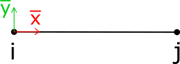
The truss element is represented schematically and can be modeled as a spring: it may only take tension or compression. Each node has two DOF, x and y. The element coordinate system has its x-axis aligned with the element direction vector going from node i to node j. Quantities with respect to the local element coordinate system are indicated by the bar over the variable.

It is considered a discrete element as opposed to a continuum element which has its variables governed by differential equations.

With the element having constant properties A (area), E (elastic modulus), and an inferred length from the nodes, L, the element stiffness in the axial direction is:

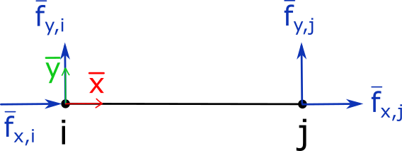
\begin{equation*} k = \frac{AE}{L} \end{equation*}

Since the element may only take tension or compression, elemental y axis forces do not contribute to member stiffness. Thus, force equilibrium and force-displacement relations become:

\begin{equation*} \bar{f} = k\Delta x = \frac{AE}{L} (\bar{u}_{x,j} - \bar{u}_{x,i}) \end{equation*}

where \(\Delta x\) is the elongation of the bar, equal to \(\bar{u}_{x,j} - \bar{u}_{x,i}\)

Then, force equilibrium requires:

\begin{equation*} -\bar{f}_{x,i} = \bar{f}_{x,j} \end{equation*}

The local element stiffness equations are then as follows:

\begin{equation*} -\bar{f}_{x,i} = \frac{AE}{L} (\bar{u}_{x,j} - \bar{u}_{x,i}) \qquad \text{or} \qquad \bar{f}_{x,i} = \frac{AE}{L} (- \bar{u}_{x,j} + \bar{u}_{x,i}) \end{equation*}

\begin{equation*} \bar{f}_{x,j} = \frac{AE}{L} (\bar{u}_{x,j} - \bar{u}_{x,i}) \end{equation*}

Which can be combined into matrix form, \(\mathbf{\bar{F}} = \mathbf{\bar{K}}\mathbf{\bar{U}}\):

\begin{equation*} \begin{bmatrix} \bar{f}_{x,i} \\ \bar{f}_{y,i}\\ \bar{f}_{x,j}\\ \bar{f}_{y,j} \end{bmatrix} = \frac{AE}{L} \begin{bmatrix} 1 & 0 & -1 & 0 \\ 0 & 0 & 0 & 0\\-1 & - & 1 & 0\\ 0 & 0 & 0 & 0\end{bmatrix} \begin{bmatrix} \bar{u}_{x,i} \\ \bar{u}_{y,i}\\ \bar{u}_{x,j}\\ \bar{u}_{y,j} \end{bmatrix} \end{equation*}

The 4x4 matrix with the coefficient is the element stiffness matrix in the element coordinate system, and for an individual element in the context of a collection of elements is denoted as \(\mathbf{\bar{K}}^e\).

Transformation

Transformation is needed to convert element quantities in the local element coordinate system to those in the global element coordinate system so they may be appropriately combined into global stiffness equations. The position or orientation of the element is defined by the nodal coordinates.

\begin{equation*} \mathbf{\bar{u}_{x,i}} \end{equation*}

\begin{equation*} \mathbf{\bar{u}_{y,i}} \end{equation*}

Displacement transformations may be inferred from graphical analysis.

\begin{equation*} \bar{u}_{x,i} = u_{x,i}\cos\theta + u_{y,i}\sin\theta \end{equation*}

\begin{equation*} \bar{u}_{y,i} = -u_{x,i}\sin\theta + u_{y,i}\cos\theta \end{equation*}

The equations for node j are the same as for node i.

\begin{equation*} \bar{u}_{x,j} = u_{x,j}\cos\theta + u_{y,j}\sin\theta \end{equation*}

\begin{equation*} \bar{u}_{y,j} = u_{x,j}\sin\theta + u_{y,j}\cos\theta \end{equation*}

Putting all 4 equations into matrix form, and with the helpers of \(c=\cos\theta\) and \(s=\sin\theta\), we have:

\begin{equation*} \begin{bmatrix}\bar{u}_{x,i} \\ \bar{u}_{y,i} \\ \bar{u}_{x,j} \\ \bar{u}_{y,j}\end{bmatrix} = \begin{bmatrix} c & s & 0 & 0 \\ -s & c & 0 & 0 \\ 0 & 0 & c & s \\ 0 & 0 & -s & c\end{bmatrix} \begin{bmatrix} u_{x,i} \\ u_{y,i} \\ u_{x,j} \\ u_{y,j} \end{bmatrix} \end{equation*}

Force transformations are the same as for displacement:

\begin{equation*} \begin{bmatrix}\bar{f}_{x,i} \\ \bar{f}_{y,i} \\ \bar{f}_{x,j} \\ \bar{f}_{y,j}\end{bmatrix} = \begin{bmatrix} c & s & 0 & 0 \\ -s & c & 0 & 0 \\ 0 & 0 & c & s \\ 0 & 0 & -s & c\end{bmatrix} \begin{bmatrix} f_{x,i} \\ f_{y,i} \\ f_{x,j} \\ f_{y,j} \end{bmatrix} \end{equation*}

The 4x4 matrix used here is the transformation matrix and is denoted as \(\mathbf{T}^e\). Conversion of quantities from the global coordinate system to the element coordinate system is done by:

\begin{equation*} \mathbf{\bar{U}}^e = \mathbf{T}^e \mathbf{U}^e \end{equation*}

\begin{equation*} \mathbf{\bar{F}}^e = \mathbf{T}^e \mathbf{F}^e \end{equation*}

Global Equations

Generation of global equations is developed by first setting equal the equations for the local element on a force basis, which yields:

\begin{equation*} \mathbf{\bar{F}}^e = \mathbf{\bar{K}}^e \mathbf{\bar{U}}^e \end{equation*}

and is equal to:

\begin{equation*} \mathbf{T}^e\mathbf{F}^e = \mathbf{\bar{K}}^e \mathbf{T}^e\mathbf{U}^e \end{equation*}

Next, both sides are multiplied by \((\mathbf{T}^e)^{-1}\), which for this element type is also equal to the transpose, \((\mathbf{T}^e)^T\):

\begin{equation*} (\mathbf{T}^e)^T \mathbf{T}^e \mathbf{F}^e = (\mathbf{T}^e)^T \mathbf{\bar{K}}^e \mathbf{T}^e \mathbf{U}^e \end{equation*}

which becomes,

\begin{equation*} \mathbf{F}^e = (\mathbf{T}^e)^T \mathbf{\bar{K}}^e \mathbf{T}^e \mathbf{U}^e \end{equation*}

therefore, the element's stiffness matrix in global coordinates is:

\begin{equation*} \mathbf{K}^e = (\mathbf{T}^e)^T \mathbf{\bar{K}}^e \mathbf{T}^e \end{equation*}

References

Introduction to Finite Element Methods (ASEN 5007). University of Colorado at Boulder. http://kis.tu.kielce.pl/mo/COLORADO_FEM/colorado/Home.html.
J. N. Reddy, Ph.D. Introduction to the Finite Element Method, Fourth Edition. Analysis of Trusses, Chapter (McGraw-Hill Education: New York, Chicago, San Francisco, Athens, London, Madrid, Mexico City, Milan, New Delhi, Singapore, Sydney, Toronto, 2019, 2006, 1993, 1984). https://www.accessengineeringlibrary.com/content/book/9781259861901/toc-chapter/chapter6/section/section3