Some time ago (2016), Microsoft released the Surface Studio accompanied by a great promo video. This product is an all-in-one computer featuring an adjustable display that maintains its position at any location set by the user. The hinge used with it - termed a "zero gravity" hinge - allows for this free positioning of the display and here we will attempt to analyze this type of design and determine how it works.
Design Notes
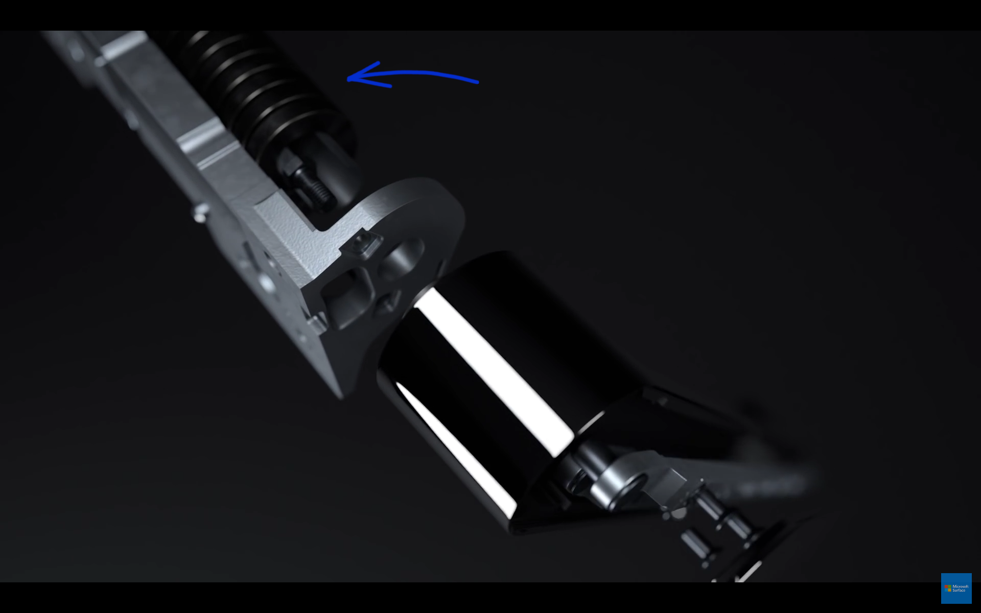
Without actually deconstructing one of these I am using images from the promo video and other publicly available information as reference.
Some observations:
- The support arms are not independent - it is a 1 degree-of-freedom (DOF) system
- Compression springs are used in the base and torsion springs are used in the display
- A four-bar linkage is used in the support arms to connect the base to the display
- This can be used to give the desired orientation response of the display by changing the lengths of the connecting members
This YouTube video confirms these observations.

Analysis
Overview
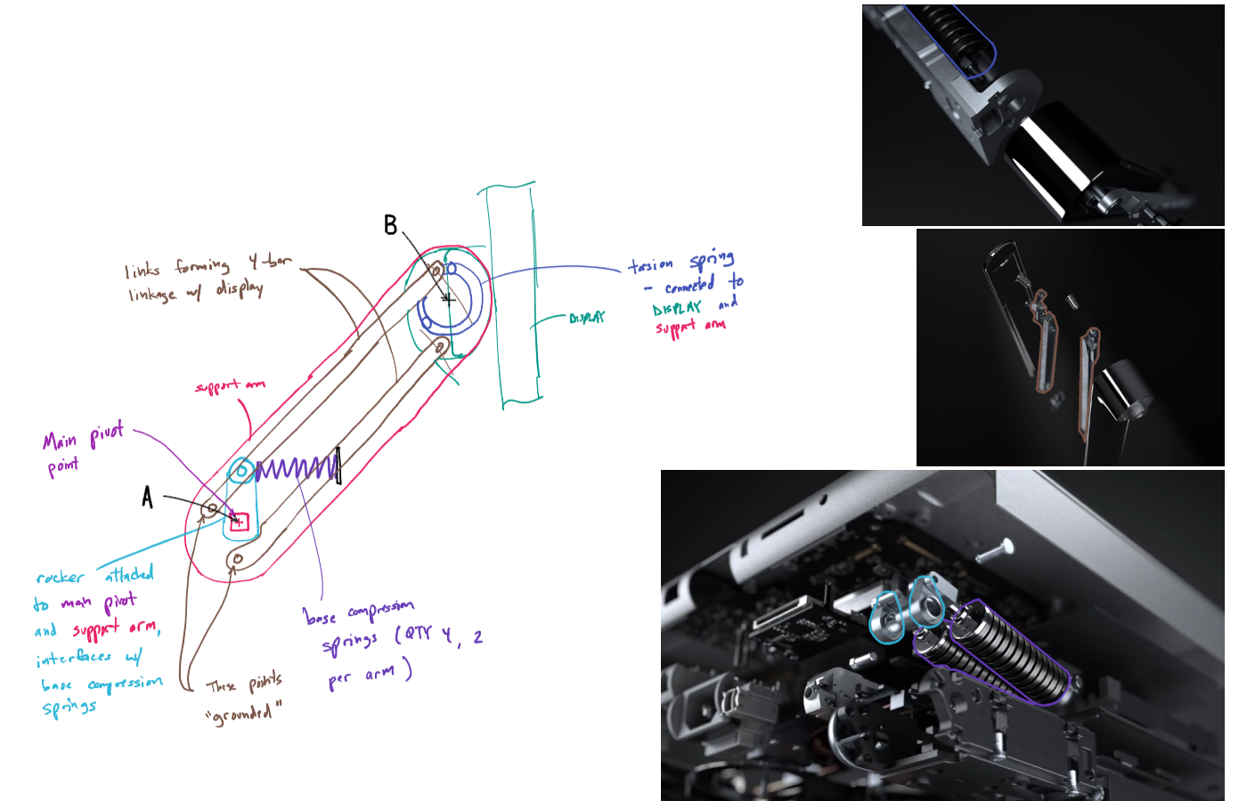
First we construct the overall layout and label relevant parts:

where,
At first glance,
- At \(B\), it appears that the moment needing resisted is only due to the display
- At \(A\), the moment due to the support arms and the display need resisted
However, since the linkage has only 1 DOF, the display would be supported (i.e. prevented from rotating) by applying a single moment anywhere along this chain such as at location \(B\) or \(A\). Thus, the moment due to the torsion spring in the display contributes to overall support of deadweight loads.
Mechanism
Based on screenshots from the above linked videos, there is a linkage (brown) internal to the two supporting arms that interfaces with compression springs in the base (purple). This linkage relates the orientation of the display with respect to the base.
Base Compression Springs
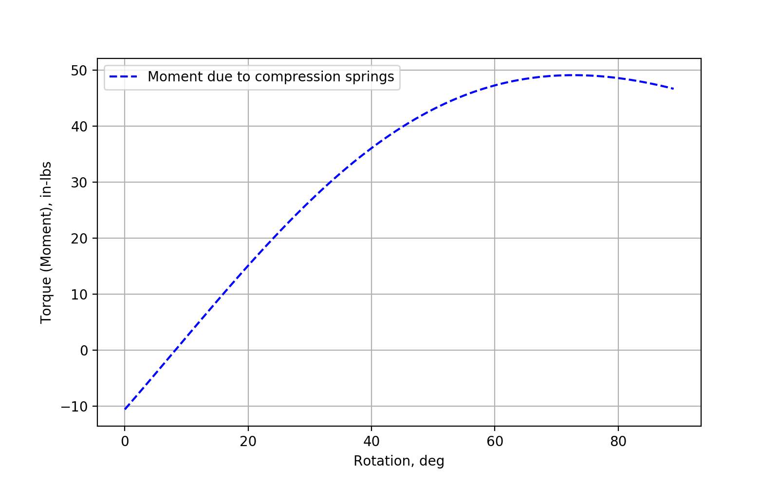
At Point A there are a total of four compression springs that act against a rocker arm (cyan). This provides a supporting moment at this joint. This moment is due to the offset height \(h\) and the spring force \(f_b=k_b\Delta l_b\). Here the moment varies non-linearly as the support arm is rotated since \(h\) changes in addition to the spring force changing.

Using the following values and properties (estimates but actually tuned to give the best result - to see if this design could work), and the accompanying Python code, this results in a moment response curve as shown below.
# Nomenclature:
#   r         = base hinge moment arm length, inches
#   r_fb      = position vector of the base of the compression spring from the
#               pivot point (Point A)
#   k_b       = spring constant of the base compression spring, lbf/in
#   l_free    = free length of the base compression spring
#   start     = start of base hinge rotation, degrees
#   end       = end of base hinge rotation, degrees
#   r_a       = Pivot arm position vector
#   r_afb     = Spring direction vector
#   u_fb      = Spring direction unit vector
#   f_b       = Spring force vector
#   M         = Moment = r x F

r = 0.3
r_fb = np.array([1.53, 0.22, 0])
k_b = 4*40
l_free = 2.5
start = 0
end = 90

spring_M, thetas = [], []

for theta in range(start,end):
    theta_rad = np.radians(theta)
    r_a = np.array([r*np.cos(theta_rad), r*np.sin(theta_rad), 0])
    r_afb = r_a - r_fb
    u_fb = r_afb/np.linalg.norm(r_afb)
    f_b = np.dot(k_b*(l_free-np.linalg.norm(r_afb)),u_fb)
    M = np.cross(r_a,f_b)

    spring_M.append(M[2])
    thetas.append(theta)

fig1, ax1 = plt.subplots()
ax1.plot(thetas, spring_M, c='b', ls='dashed',
    label='Moment due to compression springs')
ax1.grid(True)
ax1.set_xlabel('Rotation, deg')
ax1.set_ylabel('Torque (Moment), in-lbs')
Torsion Spring
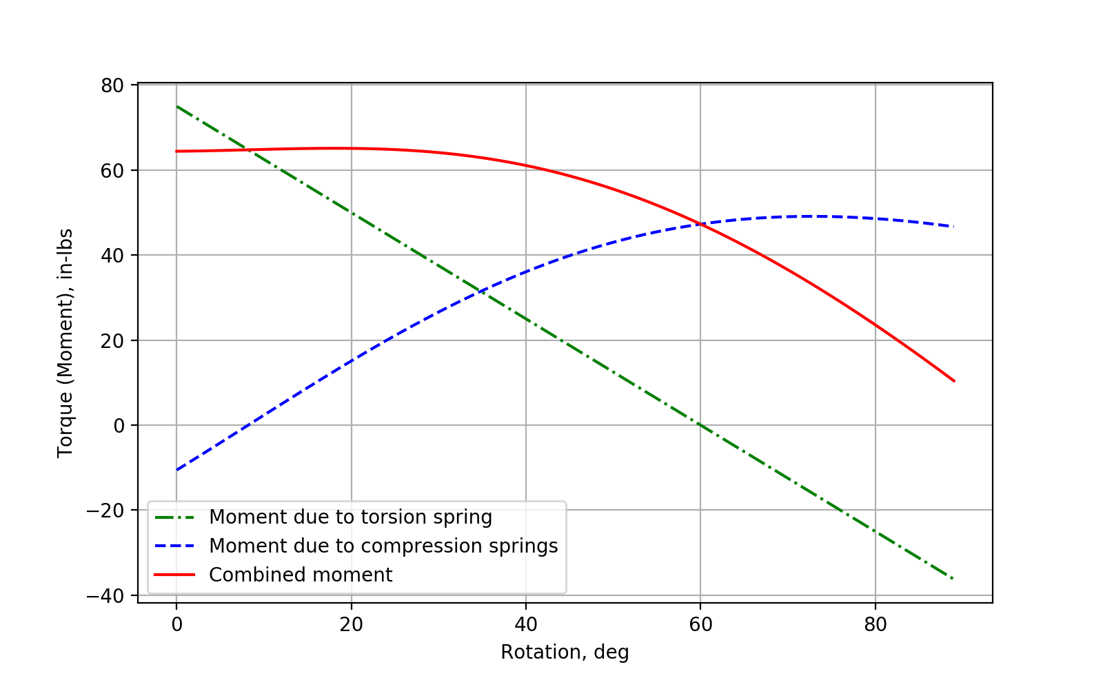
The moment due to the torsion spring is simply linear and dependent on the torsion spring stiffness. I am assuming and using some preload on this spring as I did with the compression spring.
The following properties are used and the resulting moments plotted.
k_d = 1.25                  # spring rate, lbf-in/deg
k_d_pre = 75                # Preload amount, lbs-in

tor_sp = []

for i in range(start,end):
    tor_sp.append(-k_d*i + k_d_pre)

fig2,ax2 = plt.subplots()
ax2.plot(thetas, tor_sp, '-.', c='g', label='Moment due to torsion spring')
ax2.plot(thetas, spring_M, c='b', label='Moment due to compression springs',
    ls='dashed')


# Add resisting moments of the compression springs and the torsion spring
combined = np.asarray(tor_sp) + spring_M
ax2.plot(thetas, combined, c='r', label='Combined moment')
ax2.grid(True)
ax2.legend()
ax2.set_xlabel('Rotation, deg')
ax2.set_ylabel('Torque (Moment), in-lbs')
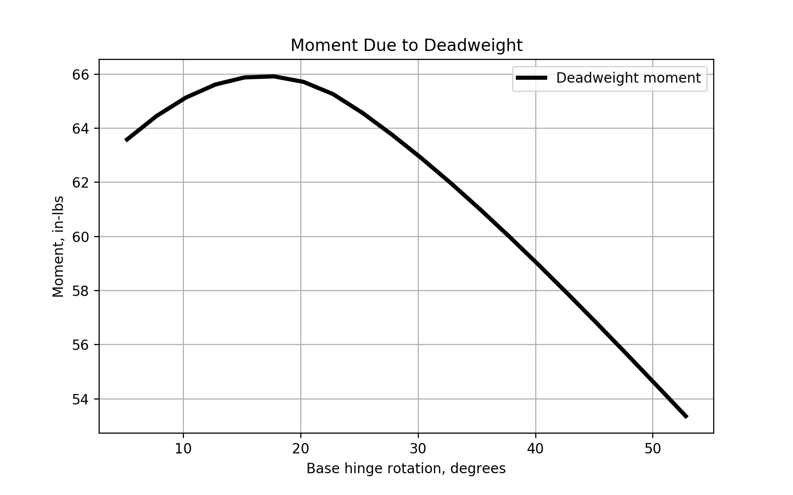
Moment at the Base Hinge From Components Due to Gravity
Now, we calculate the loads due to deadweight. The two components involved are the display and the support arms. Each is assigned a weight:
To assess if the display will be supported (or if it will fall or rise), we compare the resisting moments due to the springs to the total deadweight moment. The total deadweight moment is the resultant moment of each of the contributing moments of the display and support arms. Maintaining the display position in any configuration requires that the resisting moments and load moments be exactly equal; though small amounts of difference can be taken up through friction by the system connecting components.
Calculating the deadweight moment requires analysis of the support arm linkage. As an approximation of this we can infer the positions of the support arms and display graphically using the following screenshots:
The center of gravities are taken at the midpoint of both the support arms and display. This allows the combined moment to be estimated:
from scipy.interpolate import interp1d

# Measurement based approach - infer linkage from screenshot measurements
r_d = 3.9              # distance from display pivot point to display CG, inches
r_s = 4.0              # distance from base pivot to support arms CG, inches

m_s = 3.75             # mass of support arms, lbs
m_d = 10               # mass of display, lbs

M_dw = []              # deadweight total moment, in-lbs

# support arm and display angle measurements
disp_rot = interp1d([5.2,14.4,34.4,52.8],[142.7,132.2,115.9,96],
    kind='quadratic')
t2 = []

for theta in np.linspace(min(disp_rot.x),max(disp_rot.x),20):
    theta_rad = np.radians(theta)
    M_dw.append(
        m_s*r_s*np.cos(theta_rad)
        + m_d*(2*r_s*np.cos(theta_rad)
        + r_d*np.cos(np.radians(disp_rot(theta)))) )
    t2.append(theta)

fig3,ax3 = plt.subplots()
ax3.plot(t2, M_dw, c='black', lw=3, label='Deadweight moment')
ax3.set_title('Moment Due to Deadweight')
ax3.set_ylabel('Moment, in-lbs')
ax3.set_xlabel('Base hinge rotation, degrees')
ax3.grid(True)
ax3.legend()
fig3.savefig('fig3.png',dpi=200)

# Make a composite final figure
fig4,ax4 = plt.subplots()
ax4.plot(thetas, combined, c='r', label='Combined supporting moment')
ax4.plot(thetas, tor_sp, '-.', c='g', label='Moment due to torsion spring')
ax4.plot(thetas, spring_M, c='b', ls='dashed',
    label='Moment due to compression springs')
ax4.plot(t2, M_dw, c='black', lw=3, label='Deadweight moment')
ax4.set_ylabel('Moment, in-lbs')
ax4.set_xlabel('Base hinge rotation, degrees')
ax4.grid(True)
ax4.legend()
Moment Summary
Finally, plotting the combined moment with the deadweight moment shows reasonable agreement. More accurate properties - component weights and CG's, in addition to spring properties - would allow for better correlation but the concept confirms that this configuration can result in the desired behavior.
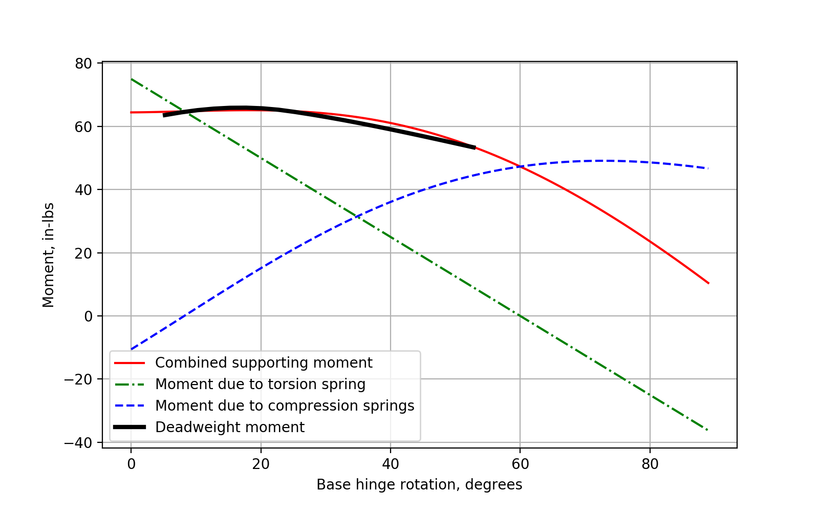
Conclusions
The configuration of springs and linkages show that equal (or near equal) moments are developed to create static equilibrium
- Friction between components could take up small differences in loads or provide for some support for the user
Tuning is accomplished primarily by selection of spring stiffenesses, spring preload amounts (i.e. the load at resting positions), length of the base hinge rocker arm, and potentially also by adjusting the weight and CG of the computer components (though less desirable than adjusting spring parameters)